Optimizing Pipelines: Controlling Concurrency in Snowflake and dbt

Intro
Hi, I’m Masa (Masa Fukui, LinkedIn), and I work as a data engineer at Nowcast (a Finatext Group company), primarily working on data pipelines that process various types of data, including job advertisement data and credit card transaction data.
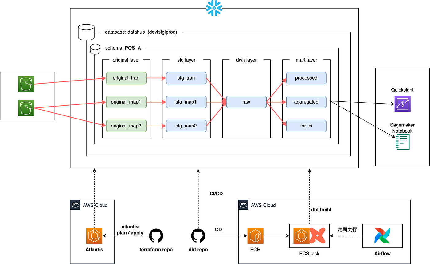
Our data infrastructure is built on Snowflake, dbt, and Airflow.
Here is a summary of this blog post:
- In Snowflake and dbt, while it is convenient to perform many operations in a single model/query using dbt macros, excessive use of macros might lead to unexpected resource issues.
- When errors occur in Snowflake due to issues such as resource exhaustion, the query profile may become unavailable. In such cases, checking the state of the Queue or Warehouse can be helpful to identify and resolve the underlying issues.
- Snowflake and dbt each have methods to control the number of concurrent query executions, which can potentially resolve issues that arise from resource contention.
As mentioned in the summary, in this blog, I will share a brief story about a performance issue we encountered in our pipelines and how we addressed it by monitoring the query queue and warehouse state in Snowflake, and controlling concurrency for our query execution. This experience also led us to review our warehouse settings and work on pipeline optimizations which in turn resulted in overall cost reduction (details to follow).
When we hear the phrase “a performance issue,” many things come to mind, but in this story, the main issues come down to:
- In our pipeline, there are cases where the data volume in the output is substantially larger than the input during query execution, leading to potential performance issues.
- Excessive resource usage in the Snowflake Warehouse, occasionally resulting in a state where even the Query Profile cannot be displayed.
Queries Where the Output Data Volume Exceeds the Input
As previously mentioned, this article focuses on the challenges arising from cases where the data volume after processing (Output) is larger than before processing (Input) in a data pipeline.
Usually, in data pipelines where big data sources such as large amounts of transaction data are involved, the data volume will often decrease after processing, resulting in Input > Output. Examples of such processing include:
- Data Selection: Selecting only the necessary columns and excluding unnecessary data from the result and the downstream.
- Filtering: Extracting only the data that meets specific conditions.
- Aggregation: Reducing the amount of data by grouping and summarizing it.
On the other hand, examples of Input < Output include:
- JOIN (especially CROSS JOIN)
JOIN involves combining data from different sources, which often results in an increase in data volume. While INNER JOIN returns only matching rows and may reduce data volume, CROSS JOIN generates all possible combinations, leading to a significant increase in output data volume.
/*
    total rows: 20,000
*/
select *
from table1 -- 100 rows
cross join table2; -- 200 rows- UNION / UNION ALL:
UNION, especially UNION ALL which does not exclude duplicates, combines the result sets vertically, often increasing the total data volume.
/*
    total rows: 300
*/
select column1, column2
from table1 -- 100 rows
union all
select column1, column2
from table2 -- 200 rows;- Melting:
Melting (un-pivoting) converts wide-format data into long-format data, often increasing the number of rows. It is often used in combination with UNION ALL in SQL.
/*
    total rows: 300
*/
select id, 'variable1' as variable, value1 as value
from table1 -- returns 100 rows
union all
select id, 'variable2' as variable, value2 as value
from table1 -- returns 100 rows
union all
select id, 'variable3' as variable, value3 as value
from table1; -- returns 100 rows
In our actual queries, we often use combinations of UNION ALL and the melt technique.
In the following section, I will demonstrate an example for this using dbt-labs’ jaffle_shop_duckdb.
Background
Before we move on, I want to elaborate on why we often write queries that result in Input < Output.
In some of the projects I am involved in, we calculate indices such as wage indices and consumption trend indices from job advertisements and transaction data, which requires complex calculations within our pipeline.
- HRog Wage Now: “Wage index” and “Job Postings Index” created from job advertisements
- JCB Consumption NOW: “Consumption Trend Index” created from credit card transaction data
Since these processes were traditionally done in Python and ran on AWS ECS, our migration to Snowflake and dbt required the extensive use of complex dbt macros and UDFs. Hence the queries introduced in the next section may not necessarily be typical in standard dbt and Snowflake pipeline development.
Example of Input < Output Queries with dbt Macros
Side Note: The jaffle_shop_duckdb provided by dbt-labs is an amazing sandbox for dbt. The only requirement is Python installed on my machine, and now I have a mini dbt sandbox running locally powered by duckdb, which comes in handy when I want to test a new version of dbt release or just want to run some experiments.
Now, let’s look at a simplified example of a query we actually run in our pipelines using dummy code. First, let’s say we have the following orders table as the input which has 99 rows. (Source)
┌──────────────────────┬─────────────┬─────────┬─────────┬─────────┬─────────┐
│     column_name      │ column_type │  null   │   key   │ default │  extra  │
│       varchar        │   varchar   │ varchar │ varchar │ varchar │ varchar │
├──────────────────────┼─────────────┼─────────┼─────────┼─────────┼─────────┤
│ order_id             │ INTEGER     │ YES     │         │         │         │
│ customer_id          │ INTEGER     │ YES     │         │         │         │
│ order_date           │ DATE        │ YES     │         │         │         │
│ status               │ VARCHAR     │ YES     │         │         │         │
│ credit_card_amount   │ DOUBLE      │ YES     │         │         │         │
│ coupon_amount        │ DOUBLE      │ YES     │         │         │         │
│ bank_transfer_amount │ DOUBLE      │ YES     │         │         │         │
│ gift_card_amount     │ DOUBLE      │ YES     │         │         │         │
│ amount               │ DOUBLE      │ YES     │         │         │         │
└──────────────────────┴─────────────┴─────────┴─────────┴─────────┴─────────┘
┌──────────┬─────────────┬────────────┬───────────┬────────────────────┬───────────────┬──────────────────────┬──────────────────┬────────┐
│ order_id │ customer_id │ order_date │ status │ credit_card_amount │ coupon_amount │ bank_transfer_amount │ gift_card_amount │ amount │
│ int32 │ int32 │ date │ varchar │ double │ double │ double │ double │ double │
├──────────┼─────────────┼────────────┼───────────┼────────────────────┼───────────────┼──────────────────────┼──────────────────┼────────┤
│ 1 │ 1 │ 2018-01-01 │ returned │ 10.0 │ 0.0 │ 0.0 │ 0.0 │ 10.0 │
│ 2 │ 3 │ 2018-01-02 │ completed │ 20.0 │ 0.0 │ 0.0 │ 0.0 │ 20.0 │
│ 3 │ 94 │ 2018-01-04 │ completed │ 0.0 │ 1.0 │ 0.0 │ 0.0 │ 1.0 │
│ 4 │ 50 │ 2018-01-05 │ completed │ 0.0 │ 25.0 │ 0.0 │ 0.0 │ 25.0 │
│ 5 │ 64 │ 2018-01-05 │ completed │ 0.0 │ 0.0 │ 17.0 │ 0.0 │ 17.0 │
│ 6 │ 54 │ 2018-01-07 │ completed │ 6.0 │ 0.0 │ 0.0 │ 0.0 │ 6.0 │
│ 7 │ 88 │ 2018-01-09 │ completed │ 16.0 │ 0.0 │ 0.0 │ 0.0 │ 16.0 │
│ 8 │ 2 │ 2018-01-11 │ returned │ 23.0 │ 0.0 │ 0.0 │ 0.0 │ 23.0 │
│ 9 │ 53 │ 2018-01-12 │ completed │ 0.0 │ 0.0 │ 0.0 │ 23.0 │ 23.0 │
│ 10 │ 7 │ 2018-01-14 │ completed │ 0.0 │ 0.0 │ 26.0 │ 0.0 │ 26.0 │
├──────────┴─────────────┴────────────┴───────────┴────────────────────┴───────────────┴──────────────────────┴──────────────────┴────────┤
│ 10 rows 9 columns │
└─────────────────────────────────────────────────────────────────────────────────────────────────────────────────────────────────────────┘In our pipeline, we use dbt macros quite extensively to perform processing which resembles the following:
-- Outer loop
{% set payment_types = [
    "credit_card",
    "coupon",
    "gift_card",
    "bank_transfer",
] %}

-- Inner loop
{% set processors = [
    "processor1",
    "processor2",
    "processor3",
] %}

{% for payment_type in payment_types %}
    {% set col_name = payment_type + "_amount" %}

    {% for processor in processors %}
        select
            order_id,
            customer_id,
            order_date,
            status,
            amount as original_amount,
            -- Call some UDF (argument: processor)
            custom_udf.process("{{ processor }}") as processed_amount,
            '{{ payment_type }}' as payment_type
        from
            {{ ref("orders") }}
        where 1=1
            and {{ col_name }} > 0

        -- Add union all if not the last iteration of the loop
        {% if not loop.last %}
        union all
        {% endif %}

    {% endfor %}

    -- Add union all if not the last iteration of the loop
    {% if not loop.last %}
    union all
    {% endif %}

{% endfor %}
Although this query is solely for demonstration purposes and the resulting data means nothing, the results will look like this, which in our case is expected by the downstream processes:
┌──────────┬─────────────┬────────────┬────────────────┬─────────────────┬─────────────────┬───────────────┐
│ order_id │ customer_id │ order_date │     status     │ original_amount │ processed_value │ payment_type  │
│  int32   │    int32    │    date    │    varchar     │     double      │     varchar     │    varchar    │
├──────────┼─────────────┼────────────┼────────────────┼─────────────────┼─────────────────┼───────────────┤
│        1 │           1 │ 2018-01-01 │ returned       │            10.0 │ xxx             │ credit_card   │
│        2 │           3 │ 2018-01-02 │ completed      │            20.0 │ xxx             │ credit_card   │
│        6 │          54 │ 2018-01-07 │ completed      │             6.0 │ xxx             │ credit_card   │
│        7 │          88 │ 2018-01-09 │ completed      │            16.0 │ xxx             │ credit_card   │
│        8 │           2 │ 2018-01-11 │ returned       │            23.0 │ xxx             │ credit_card   │
                                            .
                                            .
                                            .
Lets break down what this made-up dbt model does:
- Create nested loops with
payment_typesandprocessorslist defined using the{% set %}macro. - Use each element of these lists as a column for
payment_typeand as an argument for the made-up Snowflake UDF,processorrespectively. - In the
SELECTstatement, filter the data for each correspondingpayment_type. - Finally, add
UNION ALLto combine the result sets of each loop.
This will increases the number of rows from the original 99 to around 320. As the input grows or we introduce more processor-payment type combinations, the data volume can easily expand.
Our pipeline executes queries like the one above with large volumes of data.
While it’s possible to use intermediate tables to ease the processing load of a single model, we often use models that extensively utilize macros as they simplify code management and refactoring by keeping everything in a single model file. We wanted to keep it that way as long as no performance issues occur (foreshadowing…).
Issues Encountered in Snowflake and Queue Status
The Actual Problem We Faced in Snowflake
One day we encountered the following error while executing 4 concurrent queries in Snowflake using a dbt model which is similar to the one introduced in the previous section,
Processing aborted due to error 300005:4035471279; incident xxxxxx.As mentioned in this Snowflake KB article, this error is categorized as a Snowflake Internal Error, indicating that the memory of the warehouse has been exhausted due to excessive memory usage.
We suspected that the increase in data volume during the execution of dynamically generated queries might have led to unpredictable resource consumption pattern.
At this point, potential responses include further query optimization (possibly by using intermediate tables) or reviewing our concurrency settings. However, as mentioned earlier, we decided to first explore if we could solve the issue without changing the current code.
Query Profile Unavailable !
When there’s a problem with query execution, Snowflake’s Query Profile is a reliable tool. However, when we tried to open it, it resulted in a timeout and we couldn’t even display the profile.
In Snowflake, if a query fails due to execution timeouts for example, you can usually view the execution plan and progress up to the point of failure.
However, in our case, where a hardware failure was caused, it seems that the profile-saving process also got interrupted, rendering it unavailable.
Duration Metrics and Queue Status
With the Query Profile unavailable, we had to rely on other information, such as Duration which is available even in a case of an Internal Error.
Upon examining the details, we found that, in addition to the usual Compilation and Execution, there were also Queued Overload and Queued Repair status. The definitions for those from the official docs are as follows
QUEUED_OVERLOAD_TIME: This is the time (in milliseconds) the query spent in the warehouse queue, due to the warehouse being overloaded by the current query workload.
This status indicates that the warehouse resources are overwhelmed, causing the query to be in a waiting state.
QUEUED_PROVISIONING_TIME: The time (in milliseconds) a query waits in the warehouse queue for resources to be allocated, due to warehouse creation, resuming, or resizing.
This status indicates that the query is waiting for resources to be allocated and is also commonly seen in normal executions.
QUEUED_REPAIR_TIME: The duration (in milliseconds) that a query spends in the warehouse queue waiting for compute resources to be repaired. This situation arises when a faulty server is automatically replaced by a healthy one. This is a rare condition that can happen in the case of hardware failures.
As described, this status is rarely seen and occurs when the server fails and is attempting to recover.
As a test, we decided to run just 1 model instead of 4 to see if the queue issue would still occur and as a result we confirmed that running a single model did not lead toQUEUED_REPAIR_TIME or QUEUED_OVERLOAD_TIME.
From this information, we deduced that the resource-intensive queries running concurrently might have been causing the warehouse resources to be overwhelmed.
As each query dynamically increased the data volume, the warehouse resources became strained, leading to a situation where resources were being contended for by the queries.
Another possible explanation is that the failure occurred because the resource allocation couldn’t keep up with the unpredictable pattern of volume increase.
The Solution and Lessons Learned
Solution
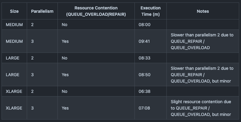
The solution was quite simple: we reduced the number of concurrent queries. Considering that the original concurrent execution with 4 concurrent queries was failing, we ran benchmarks with the following combinations:
- Warehouse sizes:
MEDIUM,LARGE,XLARGE - Number of concurrent queries:
2,3
Through these tests, we found that setting the concurrent query count to 2 prevented resource contention (QUEUED_REPAIR / OVERLOAD) regardless of the warehouse size.
Additionally, we observed that increasing the warehouse size did not linearly reduce execution time. Considering cost efficiency, running with a MEDIUM warehouse size and 2 concurrent queries seemed to be the most reasonable setup.
For our lessons learned, we initially implemented the process naively using a 2XLARGE warehouse size as we knew the query was quite resource-intensive.
However, we later discovered that it was experiencing QUEUED_OVERLOAD, resulting in unnecessarily long execution times despite not wasting credits.
By checking the queue status and benchmarking, we found that reducing the number of concurrent queries could actually shorten the total execution time, as it prevents resource contention, and led us to also reconsider the warehouse size.
In this specific case we checked the queue status in the Duration section in the query history, but with MONITOR privileges on the warehouse, you can also track the warehouse load including the queue status over time from the Snowflake Admin tab.

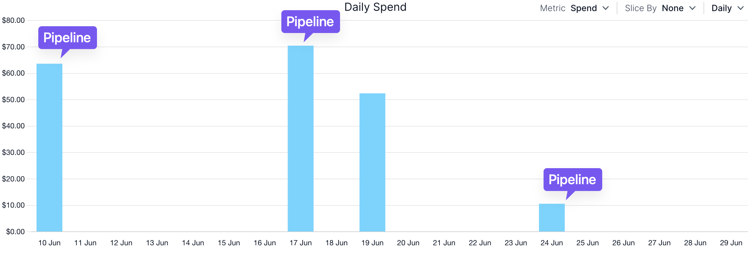
As we reduced the number of concurrent queries to 2 and changed the warehouse size from (naively chosen) 2XLARGE to MEDIUM, we were able to also reduce the overall cost of our pipeline to about one-seventh of what it was.
(The following chart was generated in SELECT.DEV)
This experience taught us the importance of not only focusing on query optimization via the Query Profile but also paying attention to the queue state and warehouse load during development and monitoring.
Going forward, we plan to incorporate queue monitoring into our routine to ensure more efficient query execution.
Controlling Concurrency in Snowflake and dbt
To conclude this article, I’d like to share a few methods for controlling concurrency in Snowflake and dbt.
Snowflake
In Snowflake, you can set and adjust the MAX_CONCURRENCY_LEVEL parameter for each warehouse.
This can be done by running the following:
ALTER WAREHOUSE MY_WAREHOUSE SET MAX_CONCURRENCY_LEVEL = 4;For existing warehouses, you can check the current settings with:
SHOW PARAMETERS IN WAREHOUSE MY_WAREHOUSE;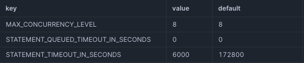
dbt
In dbt, I will introduce two methods to control concurrency:
1. --threads CLI Argument
When using the dbt CLI, you can specify the number of models to execute concurrently using the --threads option.
For example, the following command limits the maximum number of concurrently executed models to 2, regardless of how many models could theoretically be run based on their dependencies:
$ dbt run --threads 22. Forcing Dependencies
In dbt, dependencies between models are typically created using the ref macro. However, you can also manually create dependencies by adding comments to models, forcing them to run in a specific order.
For example:
-- depends_on: {{ ref('upstream_parent_model') }}

select * from {{ ref("another_model") }}We’re Hiring!
Finatext Holdings is looking for new team members! We have various engineering positions available.
For data engineers:
If you have any questions or are interested, feel free to DM me on LinkedIn!

